Climate & Weather Extremes Tutorial Climate Model Evaluation

For this first problem, you have the choice of using either NCL, Python, or both. Each NCL script in this first problem has a Python counterpart. Both scripts will make the same data files and plots. If you care about time, Python is much faster!

1. Evaluate how well the model is performing over your area of interest.

Exercise:

We want to generate a dataset that has maximum and minimum 2m Temperature (T2MAX and T2MIN) over our entire domain and one point/grid cell of interest.

1. First we want to make a file with daily max and min of T2 over the length of the model run over the entire model domain. Use the script daily_t2_maxmin.ncl (daily_t2_maxmin.py) for your exercise, you will only run the script for the months of June, July and August (we have only provided data for these months) for an eleven-year span of one of our ensemble runs.
   
   
   
   You will need to change the years we care about in the script (we want 1990-2000). Also have a look at the directories where the data files are located. You do not need to change these for the tutorial.
   
   
   
   Nothing else needs to change in the script, but it is a good idea to read the script to see what is done and get a feeling for the syntax.
   
   
   
   Run the script by typing:
   
   >ncl daily_t2_maxmin.ncl
   
   Or
   
   >python daily_t2_maxmin.py
   
   
   
   *Note: If you end up running the NCL script more than once, you will need to delete the *nc files it creates, because they will not be overwritten.
   
   
   
   This will take a about ten minutes (model data is huge!), about one minute per yearly file we create. After about a minute your first file will be finished. When it is finished, open an additional terminal window, go to your working directory and start to take a look at what is in the files you made using ncdump and ncview.
   
   
   
   ncdump is good to use to see what is in your netCDF file. This is how you use it:
   
   >ncdump –h t2_maxmin_daily_jja_1990_rtty_1990.nc
   
   
   
   ncview is useful to get a visual representation of your data in a quick and dirty way. This is how you use it:
   
   >ncview t2_maxmin_daily_jja_1990_rtty_1990.nc
   
   
   
   Also compare it to the full 365-day files that we have provided for you:
   
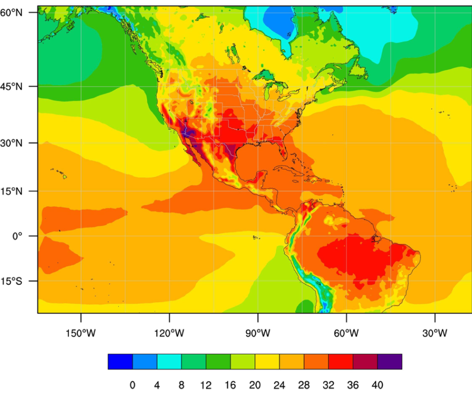
   data/t2_maxmin_daily_1990_rtty_1990.nc
2. Next, we want to make a simple spatial plot of the average of T2MAX for JJA in 1990.
   
   
   
   You will need to open the script and add in code to calculate the average. For this we are going to use the script: t2_plot.ncl (t2_plot.py)
   
   
   
   This script already reads in the daily T2MAX you created. You need to edit this script to also calculate a time average for this field.
   
   
   
   
   
   In NCL you can create an average with the following function:
   
   
   
        dim_avg_n(variable, dimension)
   
   
   
   where, variable will be the variable you want to average, and dimension is the dimension you want to average over. In our case we want to average over the first (in NCL this will be dimension 0), I.e., the time dimension.
   
   
   
   In Python you can create an average with the following function:
   
   
   
        np.ma.average(variable, axis=dimension)
   
   
   
   where, variable will be the variable you want to average, and dimension is the dimension you want to average over. In our case we want to average over the first (in Python this will be dimension 0), I.e., the time dimension.
   
   
   
   
   
   After reading in t2max, please add this line of code to create an average over JJA:
   
   NCL: t2 = dim_avg_n(t2max,0)
   
   Or:
   
   Python: t2 = np.ma.average(t2max,axis=0)
   
   
   
   Run the script by typing:
   
   >ncl t2_plot.ncl
   
   Or
   
   >python t2_plot.py
   
   
   
   You should get a plot that looks like this:
   
   
   
    

   

   
   
   
   
   Now, you can try reading and plotting the daily minimum temperature by changing all the T2MAX's in the file to T2MIN's. T2MIN is a variable in the file you made.

3. Next, because we live in the beautiful city of Boulder, CO we want to pull out the data for that point, or specifically for this case, one grid cell.
   
   We will be using the function wrf_user_ll_to_ij (or for python xy_to_ll) where we can send in a lat/lon pair and it will give us the i,j grid cell location.
   
   
   
   Also, we want to output the data in two different formats. One scientist would like it in an ascii/text file format with rows and columns. Another would like it in a netCDF file.
   
   
   
   Here we will use the larger files for the whole year that have been created for you. The paths in the scripts are correct and the only difference between the files here and the files you created in the last step are the amount of days in the file.
   
   The script we will use is time_series_point_ens.ncl (time_series_point_ens.py)
   
   The paths and time periods in the script are correct, so no edits are needed.
   
   
   
   Run the script:
   
   >ncl time_series_point_ens.ncl
   
   Or
   
   >python time_series_point_ens.py
   
   
   
   Take a look at the files that you created:
   
   t2_precip_rtty_1990.txt and t2_precip_rtty_1990.nc
   
   
   
   The files we created will be used in labs later in this tutorial on statistical downscaling and analyzing extreme events.

Let's use some of the files we created as inputs to a script that will mask out all the data outside of the areas we care about.

For this exercise, we will make use of USA State outline Shapefiles. I downloaded the ShapeFile from this website: https://www.census.gov/geographies/mapping-files/time-series/geo/tiger-line-file.2018.html, which I found with a simple Google search for US state ShapeFiles.

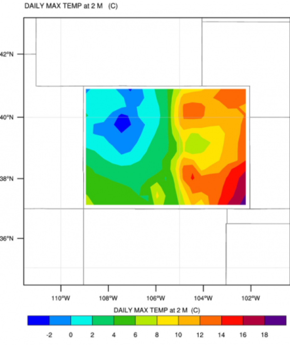
1. The script we are going to use is: >shapefile_plot.ncl
   
   
   
   We are using ShapeFiles to mask out the data outside of our area of interest. This script is set up to run without changes, but do look at the script to see what it does. Note that we are plotting data for Colorado.
   
   Run the script as before, and you should have a plot that looks like this:
   
    

   

   You can play around with the script and plot different States/Regions if you choose to do so. Or try and plot more than one state. You can also try to change the variable to plot the minimum temperature

2. Next we will use a shapefile to write the data in our area of interest to a netcdf output file. The netcdf file will have t2max and t2min with three dimensions, the year, the Julian day, and the data from each grid cell in our area of interest.
   
   
   
   Use the script shapefile.ncl to make an output file using the file you made of t2max and t2min for June, July, and August for our eleven-year period.
   
   
   
   In this file 365 is hard coded in there for the amount of days we want for each year. To make our abbreviated version work, we need to change all the 365s in the file to 93 (amount of days of our three months per year)
   
   
   
   Run the script:
   
   >ncl shapefile.ncl
   
   
   
   Look at your output file (t2_daily_State_Data_US_jja_rtty_1990.nc) using ncdump and ncview. Compare it to the file we have provided for you with the data for the entire model run (located in data/t2_daily_State_Data_US_rtty_1990.nc)

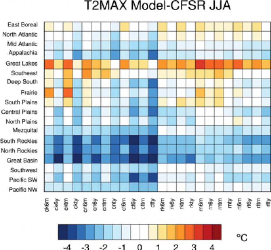
With this example we will make a difference map of a JJA T2MAX average using regional shapefile data from the 24-member physics ensemble. It compares each ensemble member to a reanalysis dataset.

To start with, the data that we have is for all 365 days of the year and we only care about JJA. Instead of subsetting in NCL, let’s use netCDF Operators (NCO) to subset the data and make new files that just have JJA in them.

netCDF Operators are extremely useful command line operators that allow for file manipulation and simple calculations. More information can be found here: http://nco.sourceforge.net

We will be using the operator ‘ncea’ to pull out JJA from the files. This is an example:

>ncea -F -d JulianDay,152,243 t2_daily_Regional_Data_rtty.nc

I have built a simple csh script that loops through all the ensemble members and makes new files.

Look at and run the script:

>./subset_jja.csh

Now that we have files with just JJA we can make the map.

This is the script:

>corrmap_t2.ncl

You need to change the names of the input files to match the names of the files that we just made. Once you make the changes, run the script:

>ncl corrmap_t2.ncl

You will get a plot that looks like this:

You can also try plotting T2MIN. T2MIN is a variable in the new files that you made.

1. Here, we would like to make a time series to see how well the model simulated the annual cycle of t2max and t2min over our area of interest (Colorado).
   
   
   
   We have provided a netCDF shapefile for you made with CFSR data. It is in the same format as the netCDF files we made before. This file is named t2_daily_State_Data_US_cfsr.nc and is located in the data directory.
   
   
   
   The files contain min and max daily temperature data for Colorado for 11 years. The data dimensions are (Years, Julian Days, grid points over Colorado)
   
   
   
   Run the script:
   
   >ncl time_series.ncl
   
   
   
   This script creates an average over both Years and Colorado area (NCL dimensions 0 and 2) to create a on dimensional average of each Julian day over the 11-year period and over the area of interest. We will be using the full years worth of data for each year here instead of the summer data we created earlier.
   
   Have a look at the plot and see if you can figure out where and how the average is created. Do you know why we used dimensions 0 and 1 to create the average and not 0 and 2 as mentioned above?
   
   
   
   Your plot should look like this: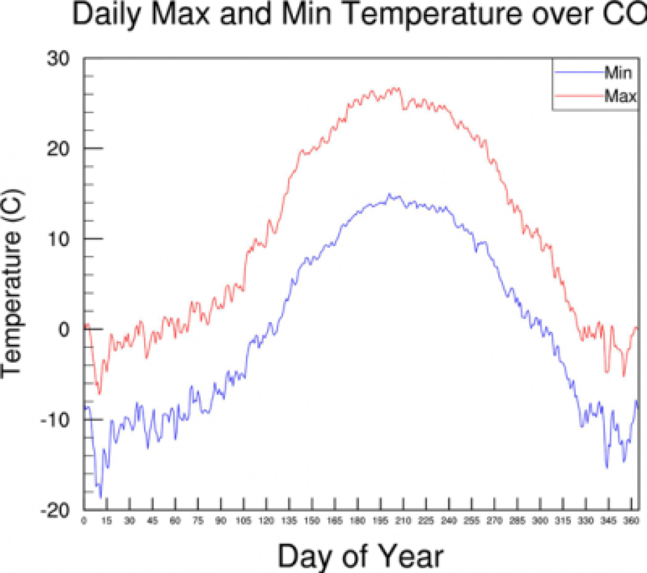

   

   Now let's add t2max and t2min from cfsr to the time series plot so we can compare it to our model run.
   
   
   
   HINTS:
   
   1. The data you want to read in is in the file: data/t2_daily_State_Data_US_cfsr.nc
   
   2. The variable names are also T2MAX_Colorado and T2MIN_Colorado
   
   3. The data in this file are in Kelvin, while the model data is in Celsius (Tk = Tc+273.15)
   
   4. Remember to also change the line information for the plot.
   
   
   
   The plot you make should look something like this: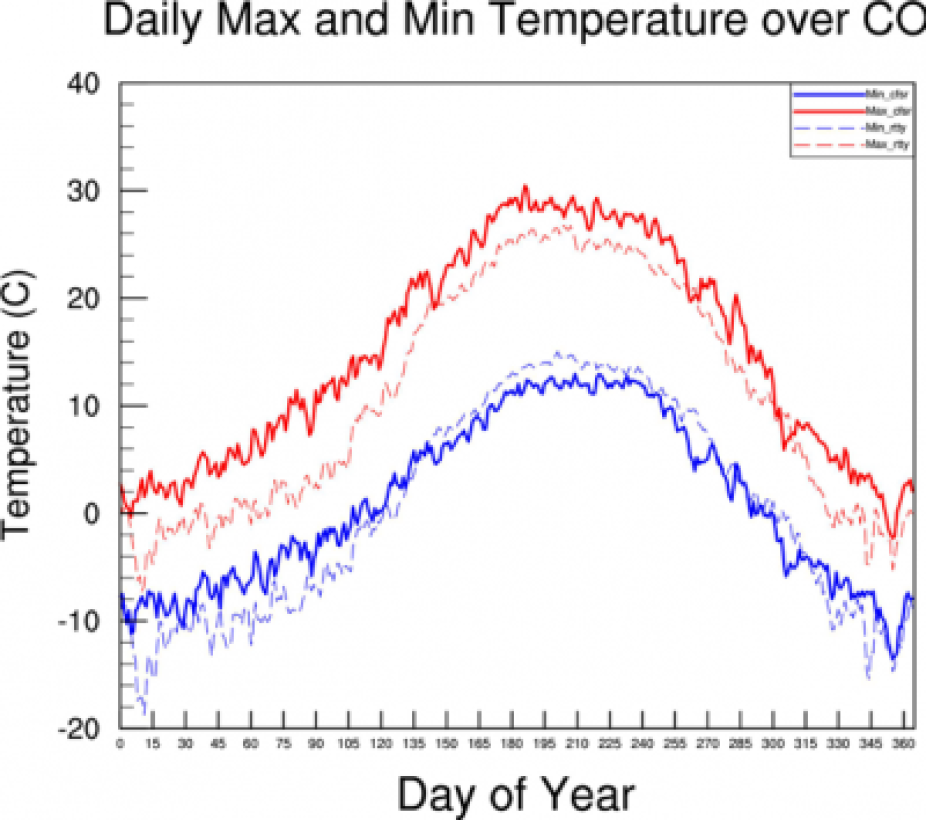

   

   If you need help, you can check out the script located here: extra/time_series_cfsr.ncl

2. Next let’s see what a monthly average looks like. The main difference is with the following lines:
   

   t2maxmon = new((/11,12,266/),float)
   t2maxjan = t2max_co(:,0:30,:)
   t2maxmon(:,0,:) = dim_avg_n(t2maxjan,1)
   
   
   t2maxdec = t2max_co(:,334:364,:)
   t2maxmon(0,11,:) = dim_avg_n(t2maxdec,1)
   

   
   
   Run the script :
   
   >ncl time_series_cfsr_monthly.ncl
   
   
   
   Please look at the script and try to understand all the differences!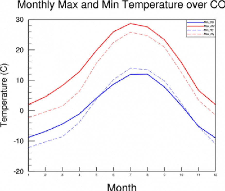

   

3. Now we will calculate and plot diurnal precipitation.
   
   
   
   *Need: We want a netCDF file that has hourly precipitation that has been averaged over Colorado for JJA.
   
   
   
   We have diurnal cycle data from 73 stations over Colorado already in ascii files located here: data/StationDataColorado_amount.txt
   
   
   
   From the model data we want to calculate three things:
   
   1. Precipitation amount: Hourly amount of any precipitation over 2.5mm
   
   2. Precipitation occurrence: How many times we have precipitation over 2.5mm in our time period (JJA).
   
   3. Precipitation intensity: Intensity (i.e. amount/occurrence)
   
   
   
   Once we have the netCDF file we will compare it to the station data that we have.
   
   
   
   The script we care about: daily_precip_jja.ncl
   
   
   
   Open up the script and go through and try to understand what is going on. I tried to put in comments to explain what is going on, but if you have questions raise your hand!
   
   
   
   Run the script:
   
   >ncl daily_precip_jja.ncl
   
   
   
   This will take a while. If you don't want to wait for it to run, you can check out the output file here: data/prec_diurnal_jja_rtty.nc
   
   The following scripts will still work if this doesn't finish running.
   
   
   
   Look at the output using ncdump -h and ncview
4. Next, we want to make a plot that compares the model data to the station data spatially.
   
   
   
   We will use the function wrf_user_ll_to_ij again to match the location with the corresponding grid cell.
   
   
   
   Look at and run the script:
   
   >ncl precip_station_diff.ncl
   
   
   
   It should show, by the hour, how the model compares to the station.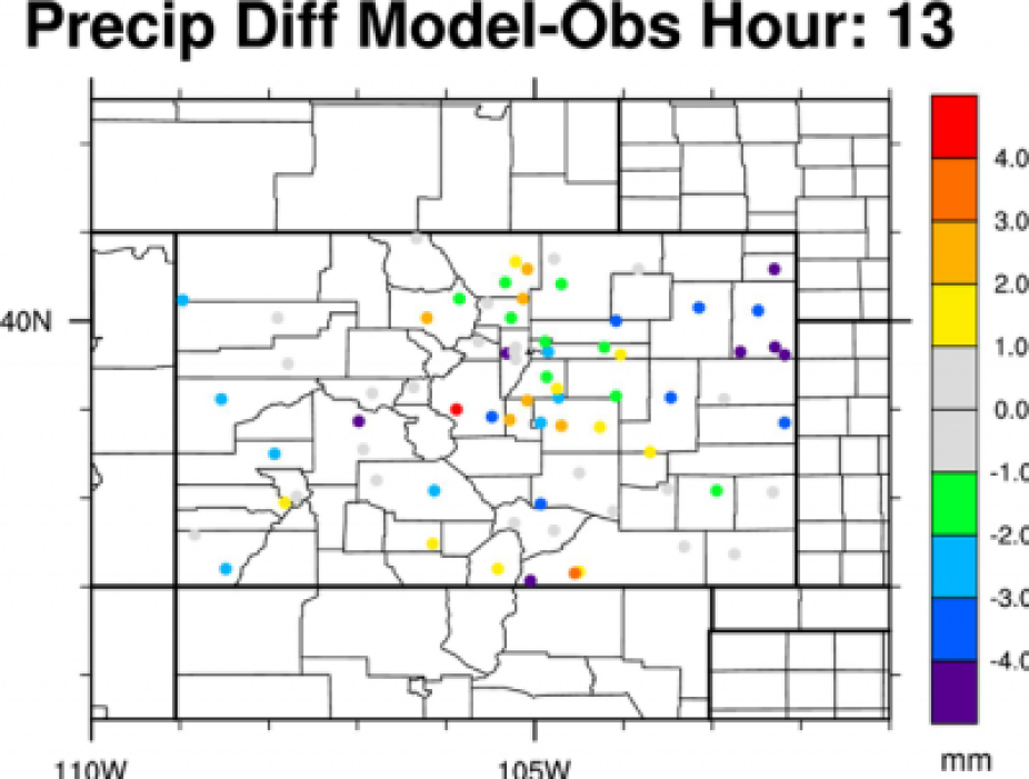

   

5. Finally, we want a plot that compares our model data and station data average over all of Colorado.
   
   
   
   Look at and run the script:
   
   >ncl precip_diurnal_panel.ncl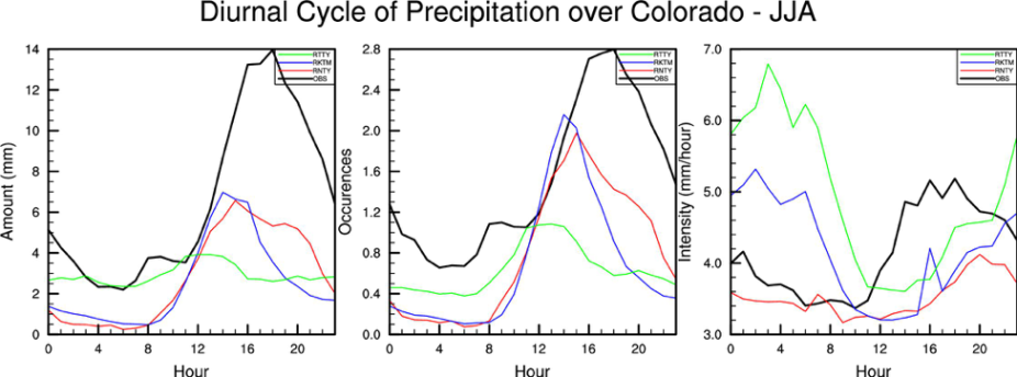

   

   Do the plots make sense to you? If you are confused, let us know!

We want to compare our model output with CFSR over Colorado using Probability Density Functions. We will compare annual T2min and T2max.

Look at and run the script:

>ncl PlotPDFs.ncl

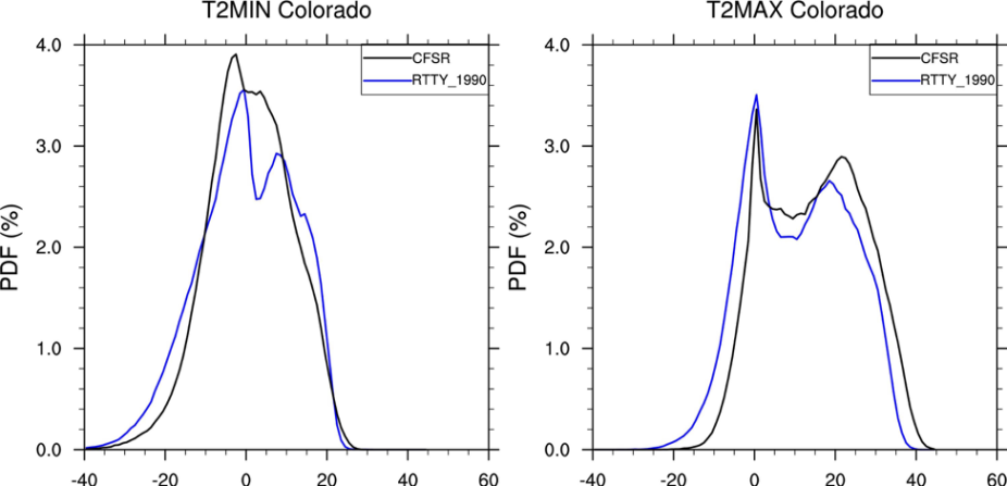
Next, we want to add in data from a future climate model run called rtty_2020

1. Make a copy of your current script:

>cp PlotPDFs.ncl PlotPDFs_2020.ncl

2. Add the PDF for rtty_2020 to the panel plot of T2MIN and T2MAX

You should get something that looks like this:

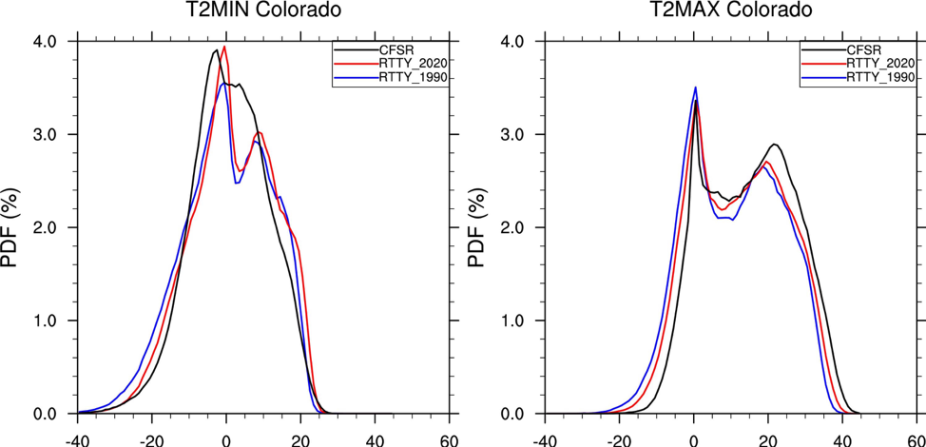
If you need help, check the extra directory for a script.

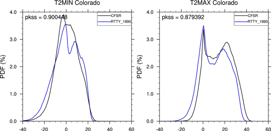
Next, we want to calculate the Perkins Skill Score, print it to the screen, and also print it on the upper left of the panels.

Use the original PlotPDFs.ncl script and make the following changes:

- After line 113 put in the following code to calculate the score:

; Perkins Skill Score
t2ens_pdfx = doubletofloat(yy(0,:)/100)
t2obs_pdfx = doubletofloat(yy(1,:)/100)
t2_perkins = new((/nBin/),float)
do i=0,nBin-1
   t2_perkins_temp = new((/2/),float)
   t2_perkins_temp(0) = t2ens_pdfx(i)
   t2_perkins_temp(1) = t2obs_pdfx(i)
   t2_perkins(i) = min(t2_perkins_temp)
   delete(t2_perkins_temp)
end do
; Sum the minimum bins to get the PSS
sum_t2_perkins = sum(t2_perkins)
; Print Perkins Skill Score to screen
print("PKSS = " +flt2string(sum_t2_perkins))

- After this line:

plots(ivar-1) = gsn_csm_xy(wks, xx, yy, res)

Put in the following code to print the score on the upper left of the panels:

; Set text size and area for Perkins Skill Score to go on upper left of panels
txres = True
txres@txFontHeightF = 0.03
amres = True
amres@amParallelPosF = -0.475
amres@amOrthogonalPosF = -0.475
amres@amJust = "TopLeft"
; Plot score on upper left of panels
txid(ivar-1) = gsn_create_text(wks,"pkss = "+flt2string(sum_t2_perkins),txres)
amid(ivar-1) = gsn_add_annotation(plots(ivar-1),txid(ivar-1),amres)

* If you need help, check the extra directory for a script.

You should get something that looks like this.

In this problem we will regrid our WRF data to the CFSR grid for comparison



NCL offers a large number of regridding functions and techniques and they can all be found here: https://www.ncl.ucar.edu/Applications/regrid.shtml



For this example we will use the function rcm2rgrid which converts a curvilinear grid to a rectilinear grid.



This is the script we care about:

Convert_WRF_to_CFSR.ncl



Regridding is intensive and can take a long time. Go into the file and change the years so that for this example we only regrid one year. This will still take some time.



Change the years on line 33 to just run for 1990.



Run the script:

>ncl Convert_WRF_to_CFSR.ncl



Use ncdump -h and ncview to look at the new file.



Your data should look like this in ncview:

For this example, we will make two different Taylor diagrams. One will compare our ensemble data to CFSR for just Colorado using the files we made using Shapefiles. The other will compare our ensemble data to CFSR over the entire domain. This will use regridded WRF data. In the regridding example in Problem 6 we made one file that was for one ensemble member for one year and it took a few minutes. I have provided the rest of the files so we don’t spend all week on this one problem.



Colorado example:

Run the ncl script:

>ncl taylor_time_co.ncl



Your plot should look like this:

DRUPAL TAG

Now, change the script to plot a Taylor diagram of T2MIN. Make sure you change each T2MAX that appears in the script to T2MIN.



Whole domain example:

Look through the script for this example and try to see all the ways we need to finesse the data, even after regridding, to compare our two data sets.

The input data for this script was calculated using the scripts from Problem 6. Each year of each ensemble member had to be regridded to match the CFSR grid.



Run the script:

>ncl taylor_time.ncl



This script takes a while, but when it finishes your plot should look like this:

DRUPALTAG

We want to run TempestExtremes over the North Atlantic and North America for both warm-core tropical cyclones and extra-tropical cyclones.

1. We will be running the feature tracker called TempestExtremes
   
   
   
   The data that will go into the tracker is the same WRF data we have been working with throughout the lab. However, I have processed it a bit more so that it would work with TempestExtremes. WRF output is not CF compliant and TempestExtremes requires all data to be CF compliant. I used this script to convert the data. I also combined the 6 hourly data into daily files and pulled out only the variables that TempestExtremes requires. Please let me know if you would like these scripts as well.
   
   
   
   Prior to running the script we need to make sure we have TempestExtremes loaded and ready to go. To do so, please run the following commands in your terminal window:
   
   
   
   >module load tempestextremes
   
   
   
   We will use a shell script named tempest-tracking.sh to run the tracker. The script is currently set up to run over all eleven years of the model ensemble. This will take about twelve minutes to run. If you do not want to wait that long, you can change the script to run just one year, which will only take about a minute. To do this, you need to change line 20 of the script to look something like this (there is data from 1990-2000):
   
    

           for f in ${PATHTOFILES}/wrfout_d01_1993*.nc
   	

   Please look at and run the script:
   
   >./tempest-tracking.sh
   
   
   
   Once it is done running it will have created a file called trajectories.txt.rtty. Open this file and take a look at it. It provides lat/lon, wind, slp and more information.
   
   
   
   Next, we will make an NCL plot of the trajectories. Please run the script:
   
   >ncl plot_traj_warm.ncl
   
   
   
   It should make a plot that looks like this (this plot is for all eleven years worth of storms):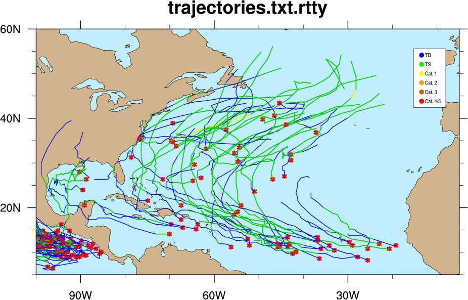

   

2. Next, we will run the tracker for extra-tropical cyclones. To do this, we need to remove the warm core test which we can do by removing the following from the line with ‘DetectCyclonesUnstructured’:
   

           ;_DIFF(Z300,Z500),-6.0,6.5,1.0
   	

   We also will need to remove the wind, latitude and terrain thresholds from the StitchNodes routine. Please remove the following text:

           --threshold “wind,>=,10.0,10;lat,<=,50.0,10;lat,>=,-50.0,10;phis,<=150.,10”
   	

   One final change you will need to make is to run the routine for only one year. Use the instructions above to change the script to only run for one year if you haven’t done so already.
   
   
   
   Finally, run the script:
   
   >./tempest-tracking.sh
   
   
   
   *If you need some help, please look at the tempest-tracking-cold.sh script in the extra/ directory.
   
   
   
   Now, make a plot of your midlatitude cyclones:
   
   >ncl plot_traj_cold.ncl
   
   
   
   You should get a plot that looks something like this: