Climate & Weather Extremes Tutorial Statistical Downscaling and Extreme Value Theory

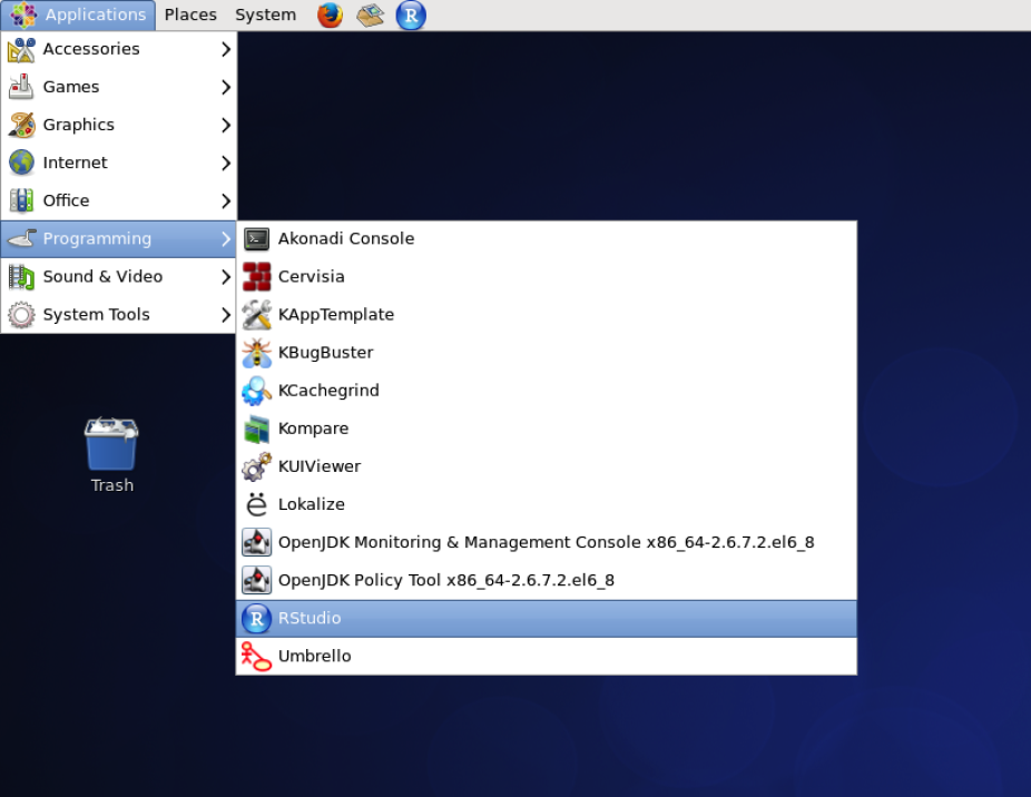
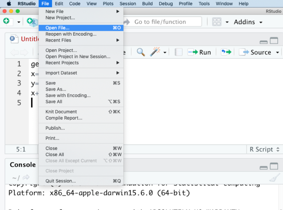
Yesterday, you manipulated your data in NCL and Python. Today, we are going to use RStudio. First step is to open RStudio:

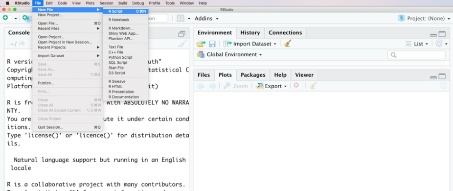
Once R Studio opens, create a new script file, shown below:

Your workspace should look like this:

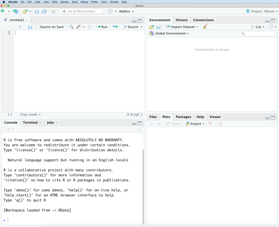
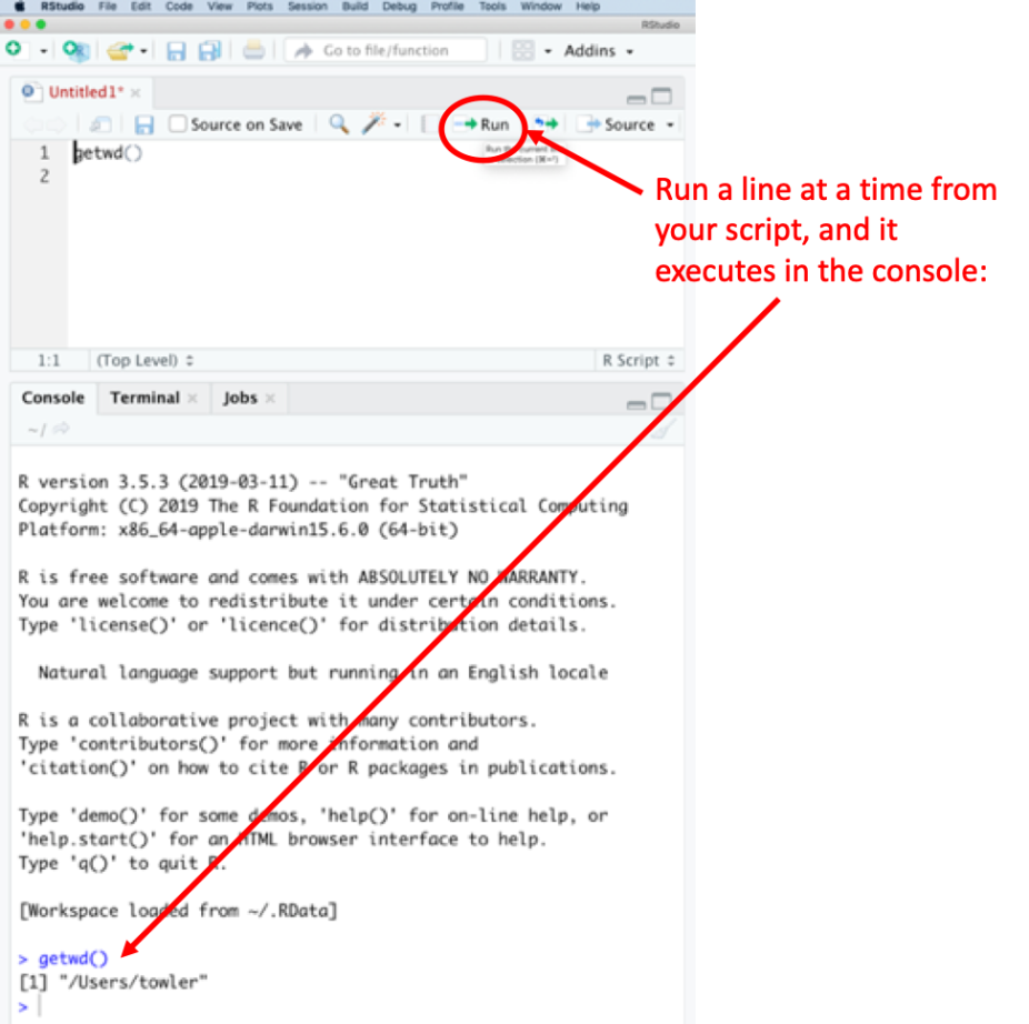
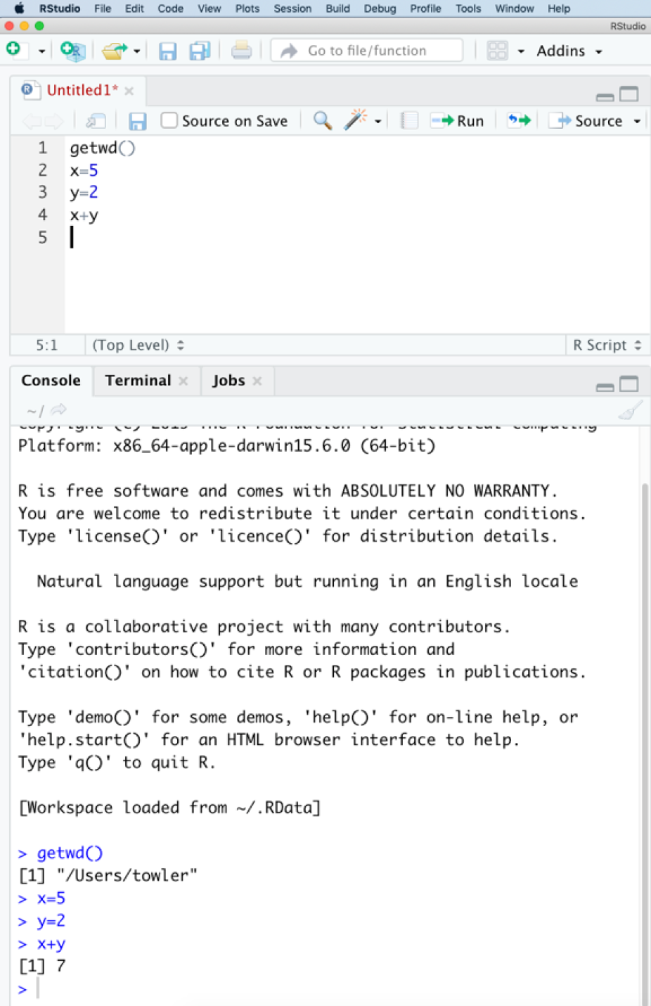
Focusing on the left two panels, the upper panel is where you can write (or load) scripts, and the lower left panel is where the commands are executed. Use the "Run" from the upper left panel to execute in the lower left, see below:

If you like, you can try typing a few commands in the script and executing them in the console:

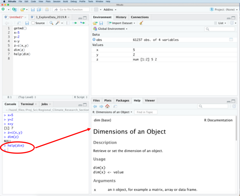
One of the most important commands is "help", if you type >help(command), it will open up documentation in the lower right corner:

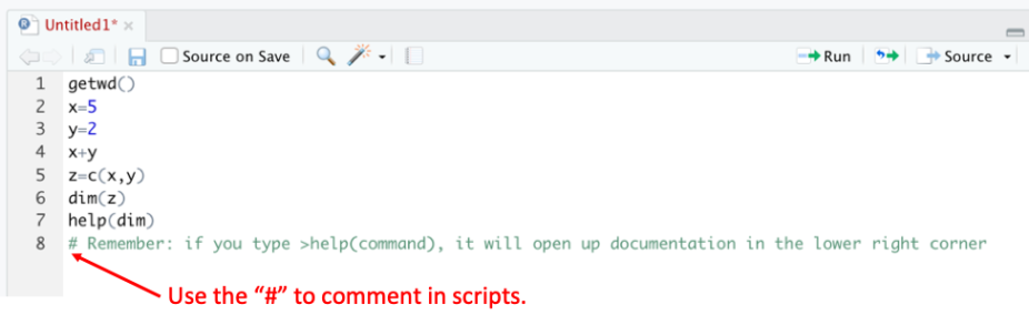
Further, as you are creating your scripts, you can use the “#” to comment:

For today’s lab, we will provide you with scripts, and you will run them line-by-line in the console, along with comments to explain each step.

Important: On the classroom machines, we need to set the working directory:

>setwd(“/sysdisk1/C3WE/statistical_downscaling”)

Once you have set your working directory, open the first code: 1_ExploreData_R.

Navigate to the file, with path: xTBDx

Now you are ready to move on to problem 2

Exercise: We want to get familiar with the observed station data from Boulder, CO. If RStudio is not open yet, please open it now, and open the script: 1_ExploreData.R. See Problem 0 if you need step-by-step instructions. The script will open in the topleft panel of RStudio. Use the Run button to run the code line-by-line, reading the code and comments as you go. The exercise has 3 “Your turns” where you will need to make changes/additions to the code, and/or answer questions based on the output. Once you complete reading and running the script, and completing the “Your Turns”, you can check your figures and answers below.

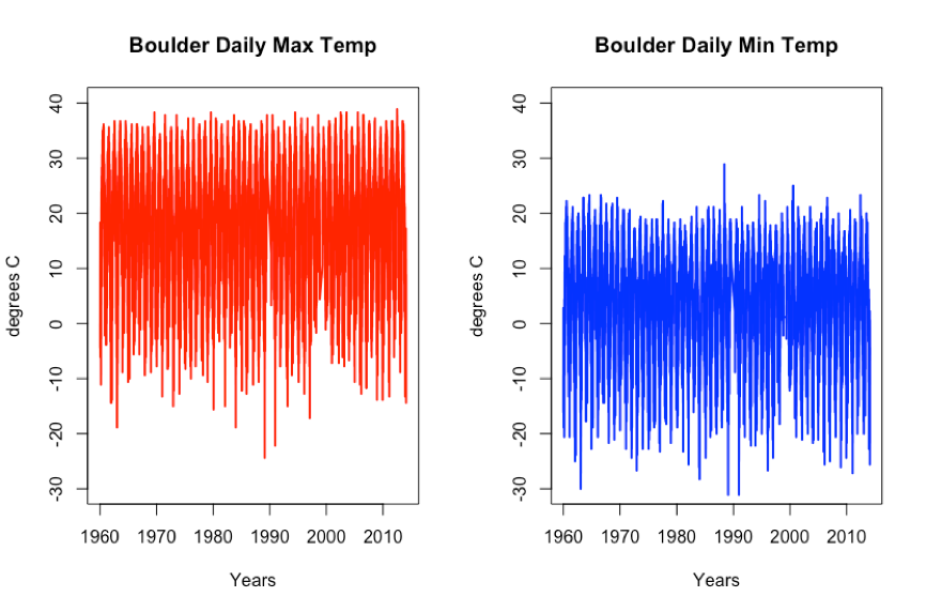
Solution: Your Turn 1. You will need to copy and paste the temperature plotting code, and make changes: change variable to “TnC” and change the color to “blue”. You should get a plot like this:

Solution to Your Turn 2: First look at the p-value from TxC:

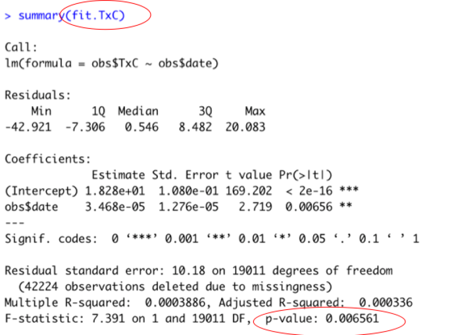
Does TxC have a statistically significant trend? (Hint: p-value of the fit needs to be <0.05).

Yes, Tmax has a significant trend; the p-value is 0.007, which is <0.05.

Next execute summary(fit.TnC), and see:

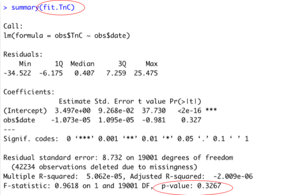
Does TnC have a statistically significant trend? (Hint: p-value of the fit needs to be <0.05).

No, Tmin does not have a temporal trend, the p-value is 0.33, which is > 0.05.

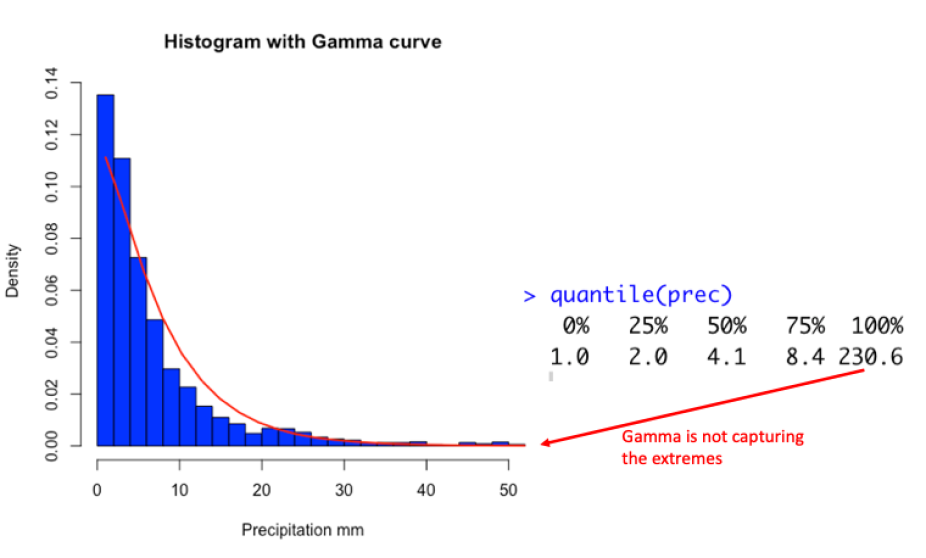
Solution to Your Turn 3.

Fitting a gamma to the daily precipitation data does not capture the extremes!

Now you are ready to move on to problem 3

Exercise: Yesterday, we extracted data from model runs over Boulder CO. Today we want to compare the observed station data to the model data from the control and future, and then compare some MOS statistical downscaling approaches. Open the script: “2_MOS_2019.R”. We provide the complete code for temperature, which you can run line-by-line, reading the comments as you go, and answering 2 “Your turns”, which you can see the answers for below. The 3^rd “Your Turn” is to repeat the exercise for precipitation. The answers for that are below as well (along with a few hints).

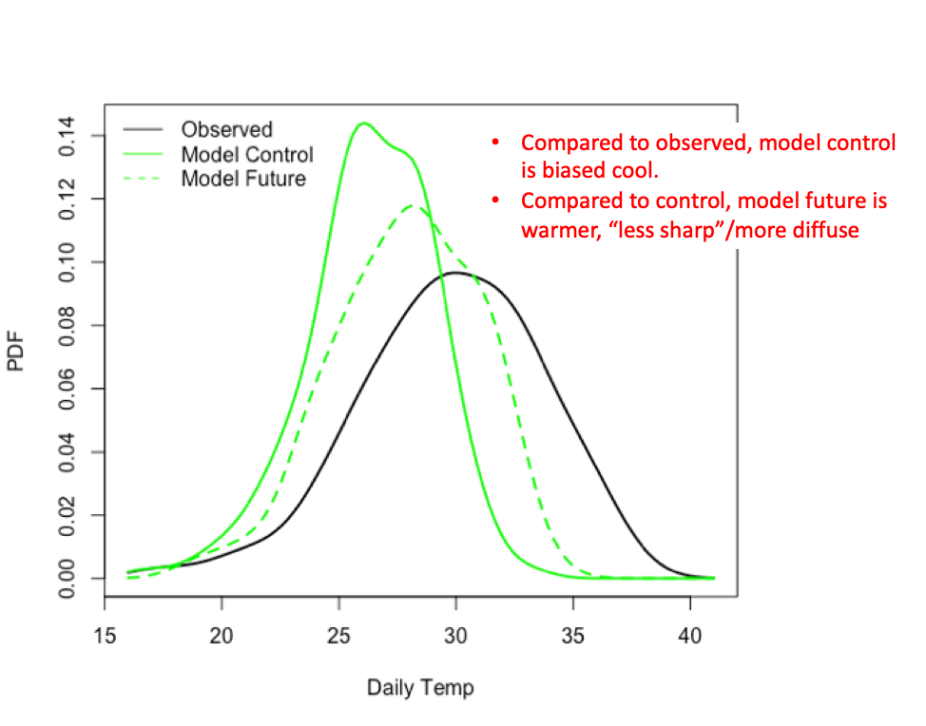
Your Turn 1. Once you plot the observed, model control, and model future, compare: (i) observed vs. model control, and (ii) model control versus model future.

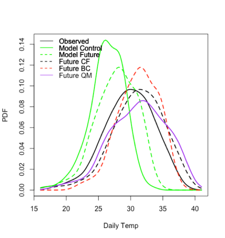
Next, when you compare three statistical downscaling methods: CF, BC, and QM for temperature. You will get a figure like this:

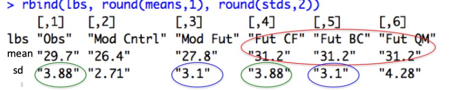
Your Turn 2: Look at the mean and standard deviations of each to compare. What do you notice as the differences, similarities between the methods:

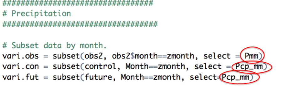
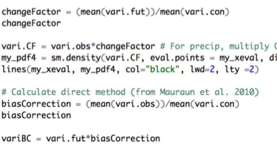
Your turn 3.: Repeat for precipitation:

And don’t forget that the equations are different for precipitation and temperature:

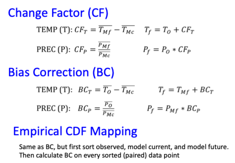
If you have trouble, see if these two code snippets help:

If you look at July (zmonth = 7), you should get a figure like this:

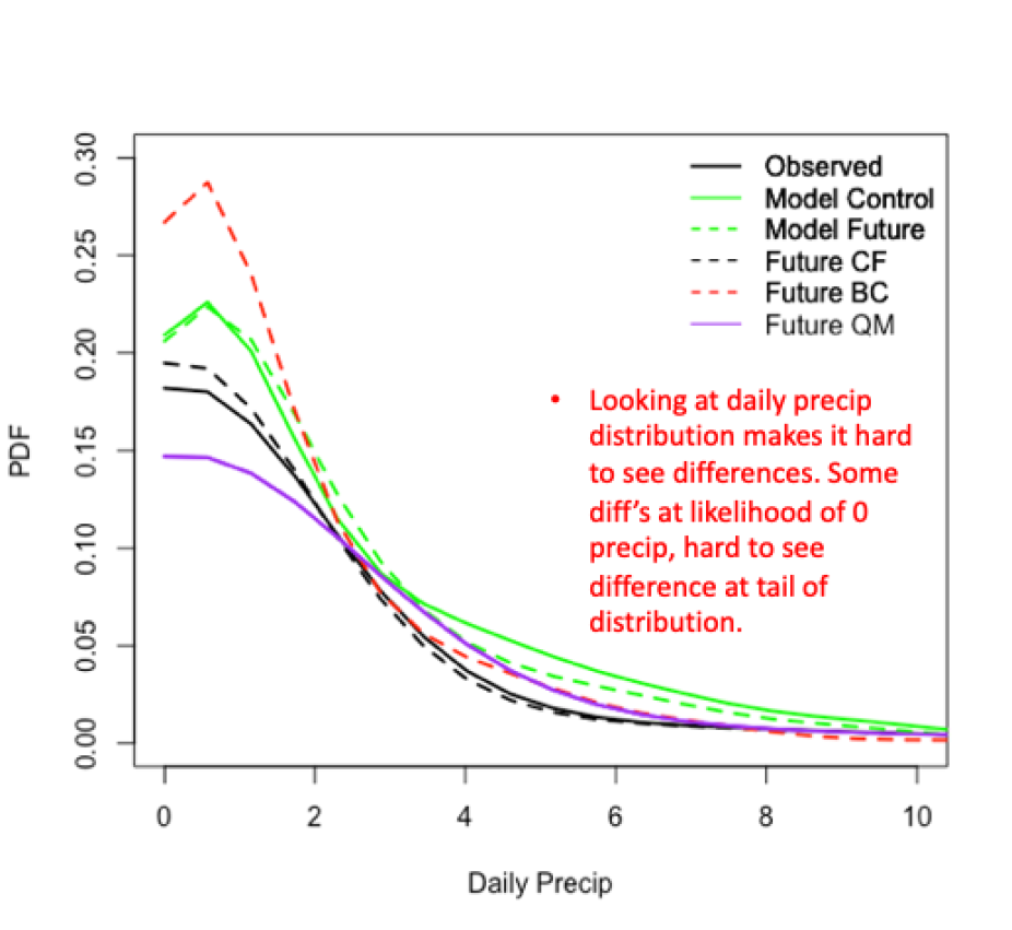
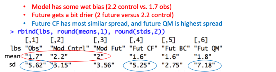
Your Turn 4: For precipitation, look at the mean and standard deviations of each to compare. What do you notice as the differences, similarities between the methods:

Now you are ready to move on to problem 4

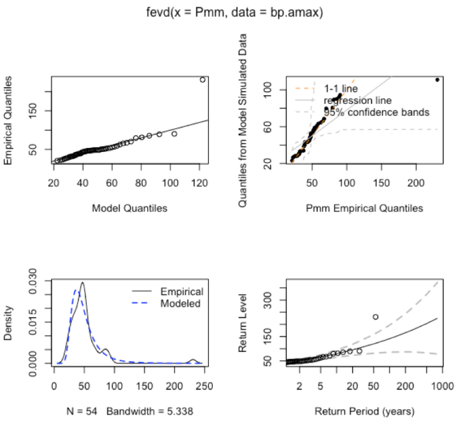
Exercise. Next, let’s turn our attention to the block maxima of precipitation. We will use years as the blocks over which to extract the maxima, and then we will fit the data using the GEV. Open Extremes_2019 code, and run line-by-line for precipitation. The first 2 “Your Turns” are questions based on the precipitation output, answers below. “Your Turn” 3 asks you to repeat for precipitation, but remove 2013. Your Turn 4 is to repeat for max temperature.

Solution: Your Turn 1: The diagnostics show that the very extreme 2013 value looks like an outlier. However, this is not uncommon for the most extreme observation, and doesn’t suggest we shouldn’t include it in the fit. Further, we see in the QQ plot it is within the 95% confidence bands, although it is outside the confidence bands for the return levels.

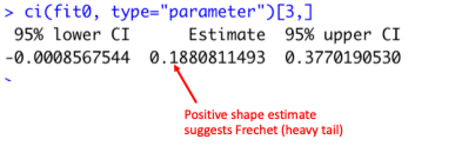
Your Turn 2: Looking at the shape parameter, the estimate is positive.

Your Turn 3: Repeat for precipitation, but to show the sensitivity of a single extreme, we remove 2013:

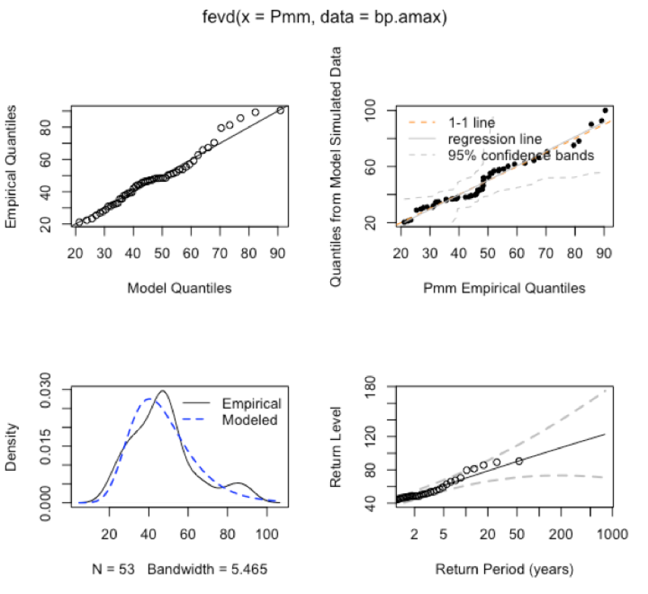
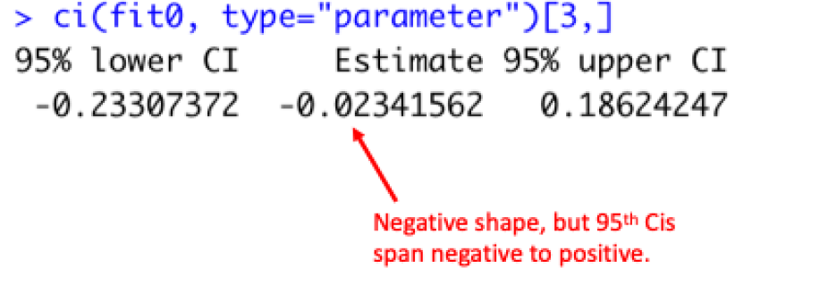
Removing 2013, the fit is tighter and the shape parameter has shifted to negative. However, the value is close to zero and the 95th CI spans from negative to positive. See Gilleland and Katz 2016 to see how to test if this is significantly different than a Gumbel (shape=0). This exercise is meant to show the sensitivity of the parameter estimates to a single extreme – i.e. if the GEV had been estimated before and after 2013. However, once it has been observed, we are not suggesting to remove very extreme data before fitting a GEV.

Your Turn 4. Repeat for maximum temperature; your plots should look like this:

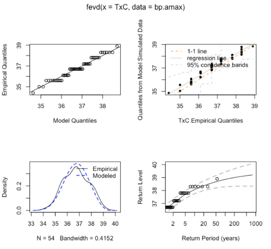
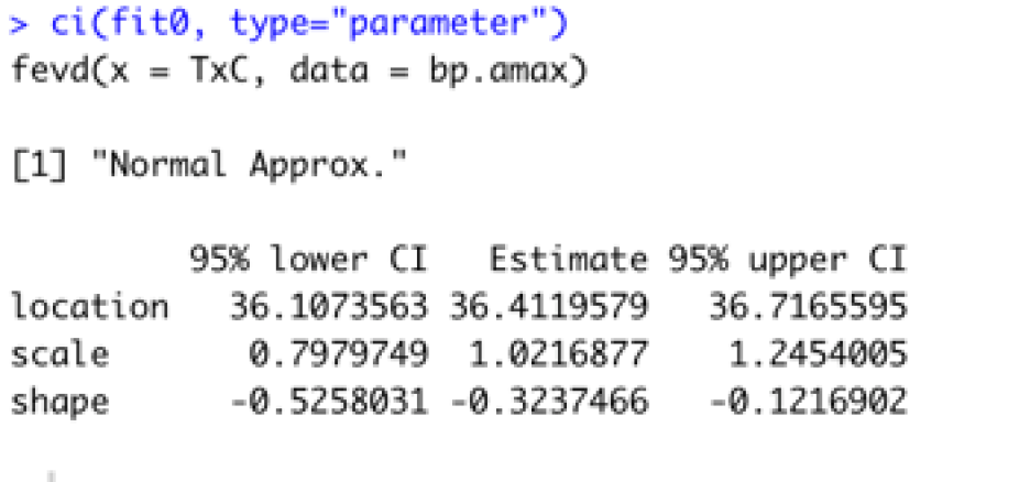
Tmax diagnostics show that the fit is reasonable, and shape parameter is negative (Weibull).

Now you are ready to move on to problem 5

Exercise: Open up Fit_Nonstationary_2019.R, run line-by-line, following the instructions in the script. There is 1 “Your turn”, solution below:

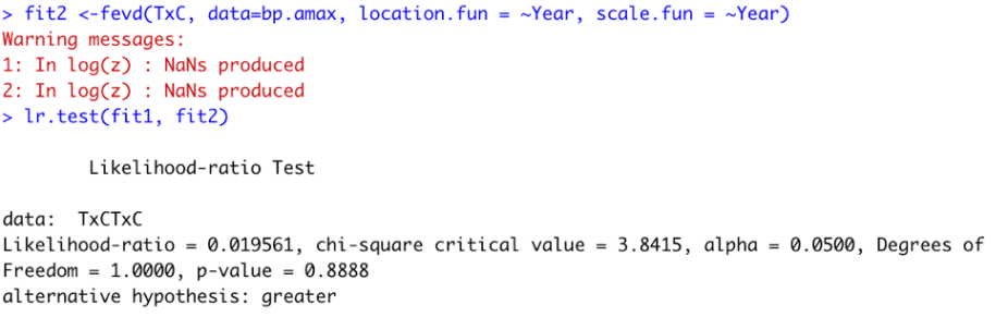
The p-value is .888, so also including the year as a covariate in the scale function does not improve the fit.

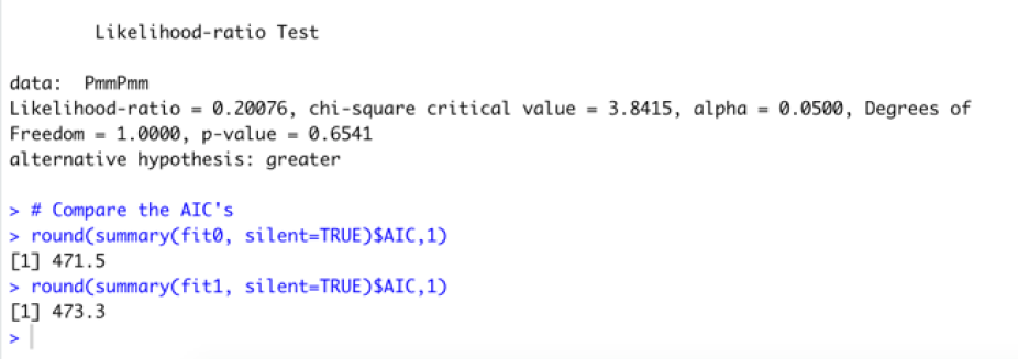
Your Turn 2: If you repeat for precipitation, you find that the temporal trend does not improve the fit:

Now you are ready to move on to problem 6

Exercise: The GEV is fit to block maxima, but the disadvantage of this is that it can waste extremes data. Here, we will fit a Generalized Pareto to peaks-over-threshold data. Open up Fit_GP_2019.R, run line-by-line, following the instructions in the script. The first “Your Turn” is to inspect the threshold diagnostic plots and to select a threshold.

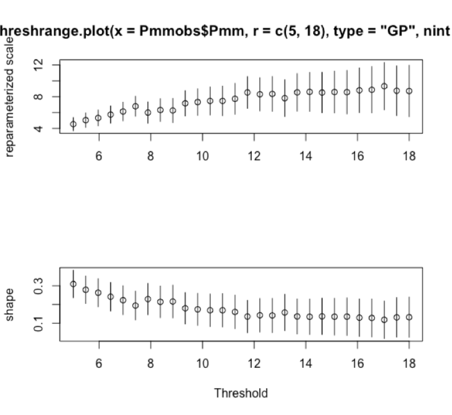
You can play around with the range and intervals (e.g., threshrange.plot(Pmmobs$Pmm, r=c(5, 18), nint=28, type="GP")). Here we illustrate selecting 8mm.

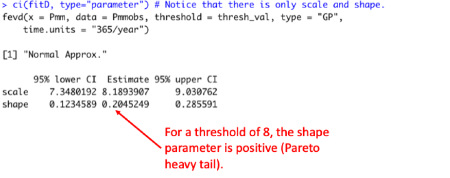
thresh_val = 8

For “Your Turn 2”, we can see that the estimate is positive, suggesting a heavy tail Pareto.

For “Your Turn 3”, we can add Year as a covariate, but it is not significant:

Congratulations, you’ve finished the Lab. Feel free to either a) load your own dataset to play around with these tools and commands or b) Look at some of the datasets and commands in Gilleland and Katz (2016): https://www.jstatsoft.org/article/view/v072i08

The latter is an excellent resource, with a variety of built-in datasets; you can follow along with the coding in the article to learn additional features of the extRemes library package.