Climate & Weather Extremes Tutorial Uncertainty

What are the relative contributions to uncertainty in seasonal tropical cyclone numbers and tropical cyclone intensity from internal variability and model physics?

Suggested Approach

Produce boxplots of seasonal tropical cyclone number and seasonal average tropical cyclone intensity (using R), to quantify and visualize the spread due to initial condition uncertainty and the spread due to model physics.

Suggested Method

* Should you need coding help, code is provided at the link at the end of this page

• Count the numbers of track files (i.e., the numbers of tropical cyclones) in the sub directories under /initial_condition_ensemble to calculate how many tropical cyclones occur in each ensemble member simulation. (Hint: use list.files and look up the help files on lapply to learn how to write and apply your own function to count the numbers of files).
• Repeat this for the physics ensemble
• Create box plots using boxplot
• Now calculate the seasonal mean tropical cyclone intensity for each ensemble member. Use variable wind10 in column 8 of the track files. Hint: use colMeans to calculate the mean intensity and loop through the files with for

After examining the box plots, which has the greatest influence on the overall uncertainty in simulated results: the model physics uncertainty or initial conditions?

Need help?

View the R code help for this question below

Note: If copying and pasting lines of code, sometimes R doesn’t like the pasted quotation marks and you may need to manually enter them in R.

setwd("/your_work_directory_path")

Question 1: What are the relative contributions to uncertainty in seasonal tropical cyclone numbers and tropical cyclone intensity from internal variability and model physics?

Create a list of names of the ensemble member subdirectories

ic_members <- list.files("initial_condition_ensemble")

Count the number of files in each subdirectory (ensemble member) using length and then concatenate them into a single file using paste.

Note: lapply applies the function and x is the list from lapply

ic_members.count <- unlist(lapply(ic_members, FUN=function(x) 
{length(list.files(paste("initial_condition_ensemble/", x,"/", sep="")))}))

physics_members <-list.files(“physics_ensemble")

physics_members.count <- unlist(lapply(physics_members,FUN=function(x) 
{length(list.files(paste("physics_ensemble/", x,"/", sep="")))}))

Print the ensemble sizes

length(ic_members.count)
# [1] 16
length(physics_members.count)
# [1] 14

Add 2 physics ensemble members (containing missing values) to make the physics ensemble the same size as the initial condition ensemble so we can make a box plot

physics_members.count <- c(physics_members.count, rep(NA, 2))

Combine the ensembles into a single array for plotting

tc.count <- cbind(ic_members.count, physics_members.count)

Make a boxplot showing the distributions of TC track counts for the initial condition and physics ensembles.

Also make the text and labels larger using cex

par(cex=1.2)
boxplot(tc.count, main="Distributions of TC Counts",
	ylab="TC count", xaxt="n")
axis(1, at=1:2, labels=c("Internal Variability", "Physics Ensemble"))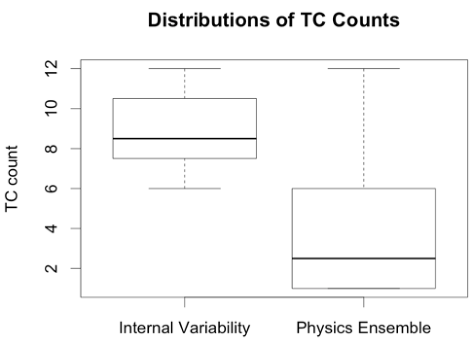

Now calculate the mean intensity for each ensemble member. Sometimes loops are unavoidable.

Create a vector

ic_members.intensity <- vector()

loop over ensemble members

for(i in 1:length(ic_members)){

list the files

file.names <- list.files(paste("initial_condition_ensemble/", ic_members[i],"/", sep=""), full.names=TRUE)

apply the function read.table to file.names to put all the track data into a data frame

track_data.df <- lapply(file.names,read.table)

Calculate the mean of column 8 (10m wind speed) for each TC track

intensity <- unlist(lapply(track_data.df, FUN= function(x){colMeans(x)[8]}))

Now calculate the ensemble mean

ic_members.intensity[i] <- mean(intensity)
}

physics_members.intensity <- vector()
for(i in 1:length(physics_members)){
file.names <-list.files(paste("physics_ensemble/", physics_members[i],"/", sep=""), full.names=TRUE)

There are missing intensity data in the physics members so we need to set the missing value

Ignore missing values when calculating the track mean intensity.

track_data.df <- lapply(file.names, FUN=function(x){read.table(x,na.strings="-999.0")})

intensity <-unlist(lapply(track_data.df,FUN=function(x){colMeans(x,na.rm=T)[8]}))
physics_members.intensity[i] <- mean(intensity)
}

Fill out the rest of the vector with missing data to be same length as physics.

physics_members.intensity <- c(physics_members.intensity, rep(NA, 2))

Combine into one data frame for plotting

tc.intensity <- cbind(ic_members.intensity, physics_members.intensity)

boxplot(tc.intensity, main="Distributions of TC Intensity",
        ylab="Intensity m/s", xaxt="n")
axis(1, at=1:2, labels=c("Internal Variability", "Physics Ensemble"))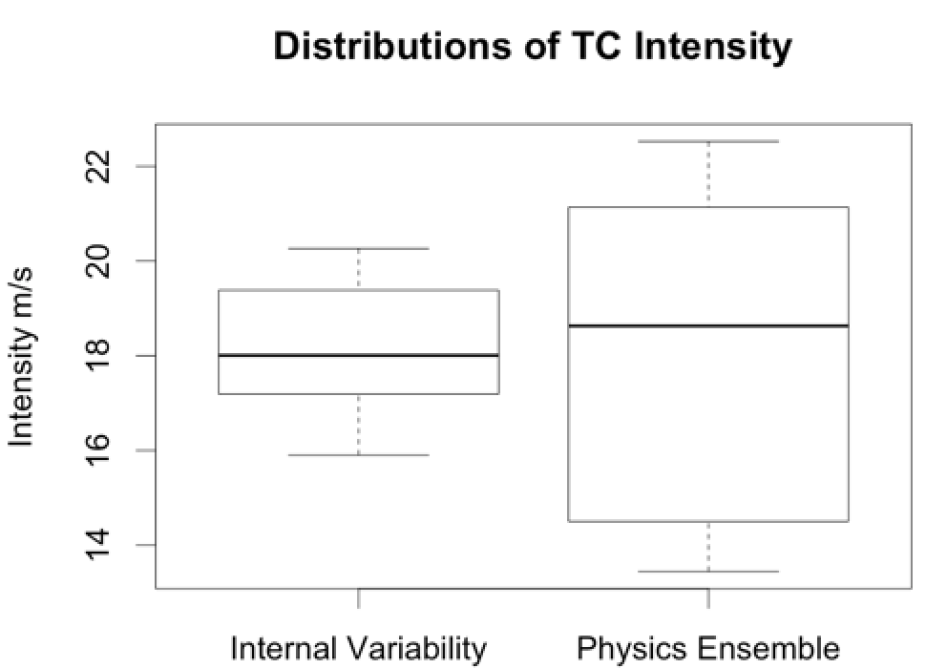

It is May 1, 1998. An insurer of shipping has exposure scattered across the North Atlantic basin. The insurer is only solvent up to 9 tropical cyclones across the basin this season. Should the insurer buy additional protection against 9 or more tropical cyclones?

Suggested Approach:

Calculate and visualize the exceedance probability of 9 tropical cyclones by fitting a distribution to the seasonal tropical cyclone numbers from the initial condition ensemble.

Suggested Method:

*Should you need coding help, code is provided at the link at the end of this page

• Fit a Poisson distribution and use this to evaluate the probability of exceeding 9 tropical cyclones in a year. Hint: use fitdistr

Need help?

View the R code help for this question below

Note: If copying and pasting lines of code, sometimes R doesn’t like the pasted quotation marks and you may need to manually enter them in R.

setwd("/your_work_directory_path")

Question 2: Calculate and visualize the exceedance probability of 9 tropical cyclones by fitting a distribution to the seasonal tropical cyclone numbers from the initial condition ensemble.

Fit a Poisson distribution to ic_members.count and use this to evaluate the probability of exceeding 9 tropical cyclones in a year.

First, need to load the package MASS to use fitdistr

library(MASS)
fit.poi <- fitdistr(ic_members.count, "poisson")

Extract the mean of the Poisson distribution (lambda)

lambda <- fit.poi$estimate

Plot a histogram of the ensemble member counts

par(cex=1.5)
hist(ic_members.count, freq=F, xlab="TC Count",
	xlim=c(0,20), col="lightblue")

Add a line for the fitted Poisson distribution

x <- 1:20
lines(x,dpois(x,lambda), lty=2, lwd=3)

Shade the area under the curve that represents the likelihood of exceeding 9 TCs.

coord.x <- c(9:20,20,9)
coord.y <- c(dpois(c(9:20),lambda),0,0)
polygon(coord.x, coord.y, col="grey")

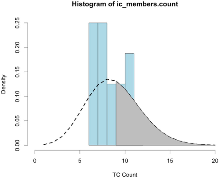
Calculate the probability of exceeding 9 TCs

1-ppois(9, lambda)
# [1] 0.3796915

How does the probability of exceedance change when considering physics uncertainty?

Need help?

View the R code help for this question below

Note: If copying and pasting lines of code, sometimes R doesn’t like the pasted quotation marks and you may need to manually enter them in R.

setwd("/your_work_directory_path")

Bonus Question 3

First, remove missing values for the physics member counts

physics_members.count <- na.omit(physics_members.count)